As part of a project that I’m completing in my masters course at university I found that I need to plot data on a map, specifically the routes of undersea cables that pass though the oceans and the depth of the sea bed. My group needed this information so that we would be able to prove that the plan we had for the product we were producing had a suitable depth rating as well as being in range of the cables we were going to be fixing.

The first big problem, getting hold of the data. To start with I played around with the data that is provided with the mapping toolbox in MATLAB for depth data but found that this wasn’t good enough for my purposes. After some hunting around the some links on MATLAB pages pointed me to the ETOPO1 1 Arc-Minute Global Relief Model were there is a download to such data in a much higher resolution than MATLAB provides. Now to plot this data.

figure
%set the map edges
latlim = [32 42];
lonlim = [5 25];

worldmap(latlim,lonlim);

[Z, refvec] = etopo('etopo1_bed_c.flt',1, latlim, lonlim);
geoshow(Z, refvec, 'DisplayType', 'surface');

demcmap(Z, 256);

This proveds me with a map within my longitude and latitude limits, which in this case are set over the central Mediterian area. This map is useful for seeing the general shape of the area, but what was important for use was defining the depths of operation, so for this i changed the final line of code:

demcmap('inc',\[0.01 -2500\],500);

This function now plots all heights above 0 (land) as one colour, then at 500 meter increments down to 2500 meters bellow mean sea level in different colours, with all depths bellow this is another colour. This allowed for the assessment of what depths the sea floor is in different areas.

The next aspect that needed to be covered was to look at ranges that could be covered from an individual port, for the early stage of research we were in we decided that we would just want to plot circles out from the port at 50 nautical mile separations, to gage the distances we would need to cover. The code to do such a task was relatively simple

%set data for Port
portlat = 37.5;
portlong = 15.083;
%add line on map for every 50 nautical miles
for x = 1:50:350
    [latc,longc] = scircle1(portlat,portlong,x,[],earthRadius('NMR'));
    plotm(latc,longc, 'black')
End

Which plotted the circles out to 350 Nautical Miles, one important point to note was this the longitude and latitude need to be in decimal format, as otherwise it won’t plot in the right location.

Next I needed to add some more data to my map, the approximate location of undersea cables, for this I used the data that is provided by Greg’s Cable Map. This is downloadable from the site and comes in either Raw File formate and KML, I downloaded it in KML as it is easy to plot such data in MATLAB, in fact it only takes one line:

geoshow('Cables.shp', 'DisplayType', 'Line', 'Color', 'r',
'MarkerEdgeColor', 'auto');

This line takes in the data file as the first argument, in this case ‘Cables.shp’, then a series of variable’s to define what it does with that data, which in this case is draw lines to represent them in red.

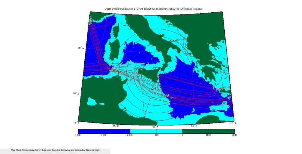
So this is the full map that I created (which includes a few extra bits not mentioned here), now to do it all around the world to pick some suitable sites for our project to be based.